Flow Metrics

A flow metric is a rule which apportions the flow passing through a cell into one or more of its neighbours.

The problem of how to best do this has been considered many times, since it is difficult to discretize flow onto a grid, and a number of solutions have been presented. Rather than choosing one, RichDEM instead incorporates many and leaves it to the user to decide which is appropriate.

Below, the various flow metrics included in RichDEM are discussed.

Wherever possible, algorithms are named according to the named according to their creators as well as by the name the authors gave the algorithm. For instance, FM_Rho8 and FM_FairfieldLeymarieD8 refer to the same function.

All flow metric functions are prefixed with !`FM_`.

Note that, in some cases, it is difficult or impossible to include a flow metric because the authors have included insufficient detail in their manuscript and have not provided source code. In these cases, the flow metric will either be absent or a “best effort” attempt has been made at implementation.

Flow Coordinate System

Internally, RichDEM refers to flow directions using a neighbourhood that appears as follows:

234
105
876

Neighbouring cells are accessed by looping through the indices 1 through 8 (inclusive) of the dx[] and dy[] arrays.

Convergent and Divergent Metrics

The greatest difference between flow metrics is in whether they are convergent or divergent. In a convergent method rivers only ever join: they never diverge or bifurcate. This means that landscape structures such as braided rivers cannot be adequately represented by a convergent method.

In a divergent method rivers may join and split, so braided rivers can be represented.

In general, convergent methods are simpler and therefore faster to use. There is a large diversity of divergent methods.

Note on the examples

Epsilon depression-filling replaces a depression with a predictable, convergent flow pattern. Beauford watershed has a number of depressions, as is evident in the example images below. A flow metric should not necessarily be judged by its behaviour within a filled depression. For convenience, a zoomed view of a non- depression area is shown and, at the end of this chapter, the views are compared.

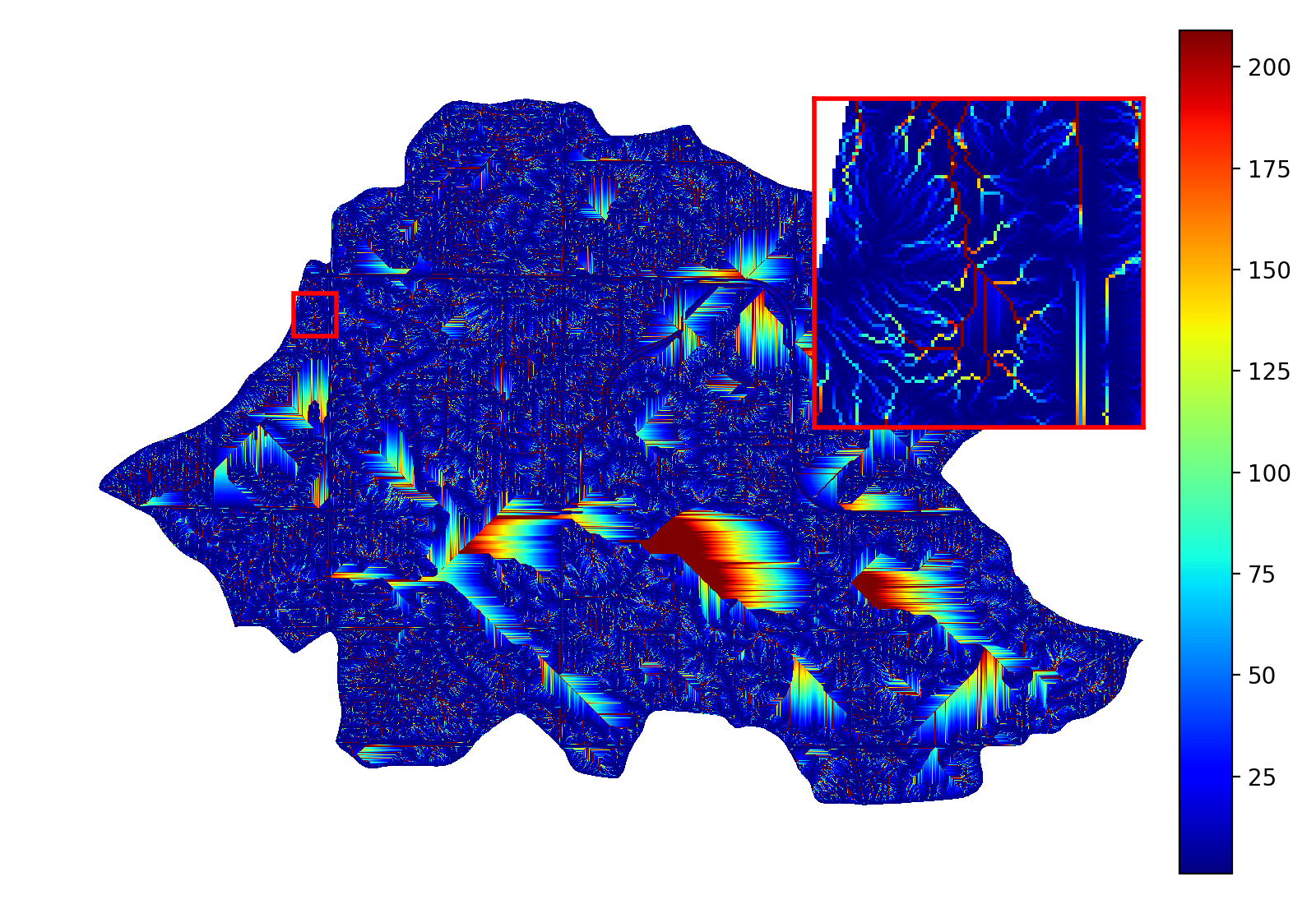
D8 (O’Callaghan and Mark, 1984)

O’Callaghan, J.F., Mark, D.M., 1984. The Extraction of Drainage Networks from Digital Elevation Data. Computer vision, graphics, and image processing 28, 323–344.

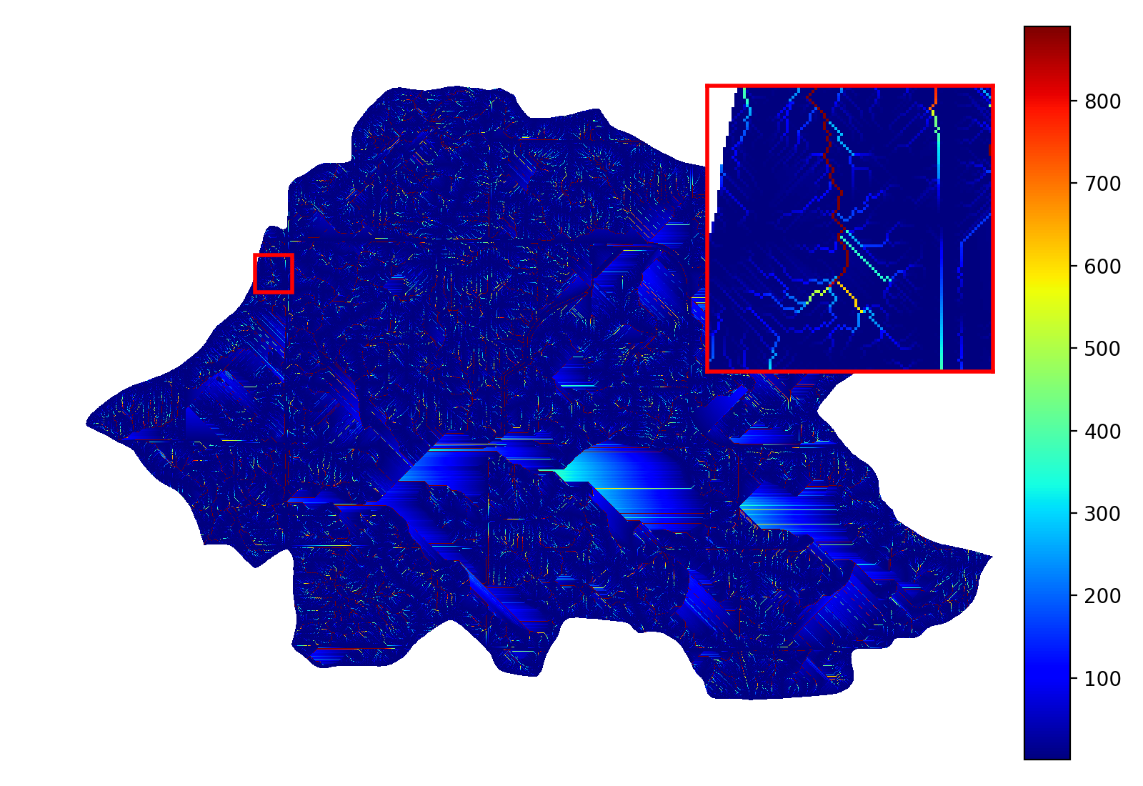
The D8 method assigns flow from a focal cell to one and only one of its 8 neighbouring cells. The chosen neighbour is the one accessed via the steepest slope. When such a neighbour does not exist, no flow direction is assigned. When two or more neighbours have the same slope, the chosen neighbour is the first one considered by the algorithm.

This is a convergent, deterministic flow method.

import richdem as rd
import numpy as np

dem = rd.rdarray(np.load('imgs/beauford.npz')['beauford'], no_data=-9999)

rd.FillDepressions(dem, epsilon=True, in_place=True)
accum_d8 = rd.FlowAccumulation(dem, method='D8')
d8_fig = rd.rdShow(accum_d8, zxmin=450, zxmax=550, zymin=550, zymax=450, figsize=(8,5.5), axes=False, cmap='jet')

(Source code, png, hires.png, pdf)

Language	Command
C++	richdem::FM_OCallaghanD8 or richdem::FM_D8()

D4 (O’Callaghan and Mark, 1984)

O’Callaghan, J.F., Mark, D.M., 1984. The Extraction of Drainage Networks from Digital Elevation Data. Computer vision, graphics, and image processing 28, 323–344.

The D4 method assigns flow from a focal cell to one and only one of its 4 north, south, east, or west neighbouring cells. The chosen neighbour is the one accessed via the steepest slope. When such a neighbour does not exist, no flow direction is assigned. When two or more neighbours have the same slope, the chosen neighbour is the first one considered by the algorithm.

This is a convergent, deterministic flow method.

import richdem as rd
import numpy as np

dem = rd.rdarray(np.load('imgs/beauford.npz')['beauford'], no_data=-9999)

rd.FillDepressions(dem, epsilon=True, in_place=True)
accum_d4 = rd.FlowAccumulation(dem, method='D4')
d8_fig = rd.rdShow(accum_d4, zxmin=450, zxmax=550, zymin=550, zymax=450, figsize=(8,5.5), axes=False, cmap='jet')

(Source code, png, hires.png, pdf)

Language	Command
C++	richdem::FM_OCallaghanD4 or richdem::FM_D4()

Rho8 (Fairfield and Leymarie, 1991)

Fairfield, J., Leymarie, P., 1991. Drainage networks from grid digital elevation models. Water resources research 27, 709–717.

The Rho8 method apportions flow from a focal cell to one and only one of its 8 neighbouring cells. To do so, the slope to each neighbouring cell is calculated and a neighbouring cell is selected randomly with a probability weighted by the slope.

This is a convergent, stochastic flow method.

accum_rho8 = rd.FlowAccumulation(dem, method='Rho8')
rd.rdShow(accum_rho8, zxmin=450, zxmax=550, zymin=550, zymax=450, figsize=(8,5.5), axes=False, cmap='jet', vmin=d8_fig['vmin'], vmax=d8_fig['vmax'])

(Source code, png, hires.png, pdf)

Language	Command
C++	richdem::FM_Rho8() or richdem::FM_FairfieldLeymarieD8

Rho4 (Fairfield and Leymarie, 1991)

Fairfield, J., Leymarie, P., 1991. Drainage networks from grid digital elevation models. Water resources research 27, 709–717.

The Rho4 method apportions flow from a focal cell to one and only one of its 8 neighbouring cells. To do so, the slope to each neighbouring cell is calculated and a neighbouring cell is selected randomly with a probability weighted by the slope.

This is a convergent, stochastic flow method.

accum_rho4 = rd.FlowAccumulation(dem, method='Rho4')
rd.rdShow(accum_rho4, zxmin=450, zxmax=550, zymin=550, zymax=450, figsize=(8,5.5), axes=False, cmap='jet', vmin=d8_fig['vmin'], vmax=d8_fig['vmax'])

(Source code, png, hires.png, pdf)

Language	Command
C++	richdem::FM_Rho4() or richdem::FM_FairfieldLeymarieD4

Quinn (1991)

Quinn, P., Beven, K., Chevallier, P., Planchon, O., 1991. The Prediction Of Hillslope Flow Paths For Distributed Hydrological Modelling Using Digital Terrain Models. Hydrological Processes 5, 59–79.

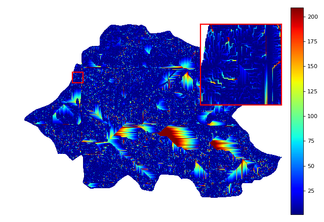
The Quinn (1991) method apportions flow from a focal cell to one or more, and possibly all, of its 8 neighbouring cells. To do so, the amount of flow apportioned to each neighbour is a function \(\tan(\beta)^1\) of the slope \(\beta\) to that neighbour. This is a special case of the Holmgren (1994) method.

This is a divergent, deterministic flow method.

accum_quinn = rd.FlowAccumulation(dem, method='Quinn')
rd.rdShow(accum_quinn, zxmin=450, zxmax=550, zymin=550, zymax=450, figsize=(8,5.5), axes=False, cmap='jet', vmin=d8_fig['vmin'], vmax=d8_fig['vmax'])

(Source code, png, hires.png, pdf)

Language	Command
C++	richdem::FM_Quinn()

Freeman (1991)

Freeman, T.G., 1991. Calculating catchment area with divergent flow based on a regular grid. Computers & Geosciences 17, 413–422.

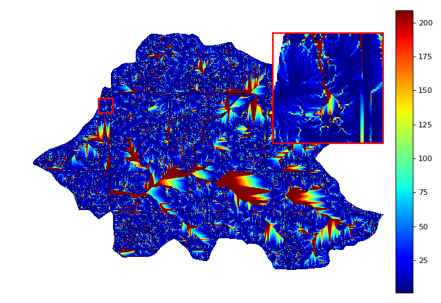
The Freeman (1991) method apportions flow from a focal cell to one or more, and possibly all, of its 8 neighbouring cells. To do so, the amount of flow apportioned to each neighbour is a function of the slope to that neighbour and a tuning parameter \(p\). In particular, the fraction \(f_i\) of flow apportioned to neighbour \(i\) is

\[f_i = \frac{\max(0,\beta_i^p)}{\sum_{j \in N} \max(0,\beta_j^p)}\]

Freeman recommends choosing \(p \approx 1.1\).

This is a divergent, deterministic flow method.

accum_freeman = rd.FlowAccumulation(dem, method='Freeman', exponent=1.1)
rd.rdShow(accum_freeman, zxmin=450, zxmax=550, zymin=550, zymax=450, figsize=(8,5.5), axes=False, cmap='jet', vmin=d8_fig['vmin'], vmax=d8_fig['vmax'])

(Source code, png, hires.png, pdf)

Language	Command
C++	richdem::FM_Freeman()

Holmgren (1994)

Holmgren, P., 1994. Multiple flow direction algorithms for runoff modelling in grid based elevation models: an empirical evaluation. Hydrological processes 8, 327–334.

The Holmgren (1994) method apportions flow from a focal cell to one or more, and possibly all, of its 8 neighbouring cells. To do so, the amount of flow apportioned to each neighbour is a function of the slope that neighbour and a user-specified exponent \(x\). In particular, the fraction \(f_i\) of flow apportioned to neighbour \(i\) is

\[f_i = \frac{(\tan \beta_i)^x}{\sum_{j \in N} (tan \beta_j)^x} \forall \tan \beta > 0\]

This is a generalization of the Quinn (1991) method in which the exponent is 1. As \(x \rightarrow \infty\), this method approximates the D8 method.

Holmgren recommends choosing \(x \in [4,6]\).

This is a divergent, deterministic flow method.

accum_holmgren = rd.FlowAccumulation(dem, method='Holmgren', exponent=5)
rd.rdShow(accum_holmgren, zxmin=450, zxmax=550, zymin=550, zymax=450, figsize=(8,5.5), axes=False, cmap='jet', vmin=d8_fig['vmin'], vmax=d8_fig['vmax'])

(Source code, png, hires.png, pdf)

Language	Command
C++	richdem::FM_Holmgren()

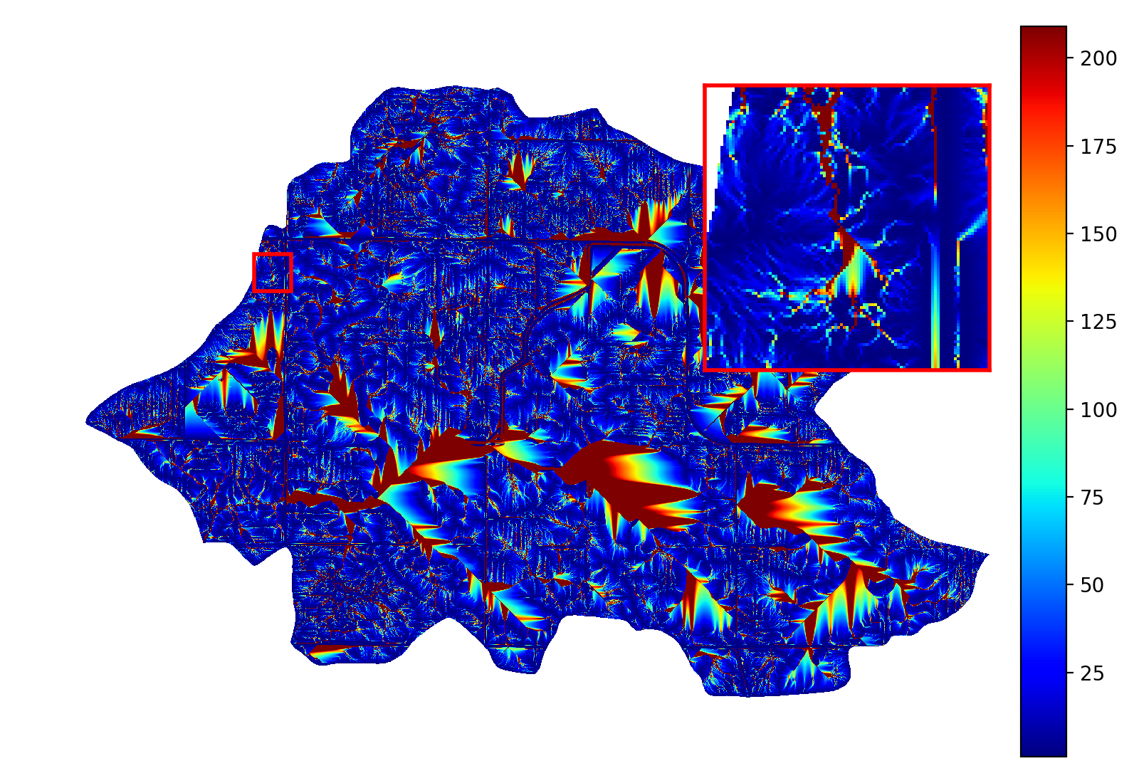
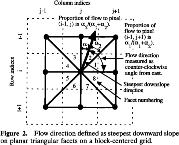
D∞ (Tarboton, 1997)

Tarboton, D.G., 1997. A new method for the determination of flow directions and upslope areas in grid digital elevation models. Water resources research 33, 309–319.

The D∞ method apportions flow from a focal cell between one or two adjacent neighbours of its 8 neighbouring cells. To do so, a line of steepest descent is calculated by doing localized surface fitting between the focal cell and adjacent pairs of its neighbouring cell. This line often falls between two neighbours.

This is a divergent, deterministic flow method.

accum_dinf = rd.FlowAccumulation(dem, method='Dinf')
rd.rdShow(accum_dinf, zxmin=450, zxmax=550, zymin=550, zymax=450, figsize=(8,5.5), axes=False, cmap='jet', vmin=d8_fig['vmin'], vmax=d8_fig['vmax'])

(Source code, png, hires.png, pdf)

Language	Command
C++	richdem::FM_Tarboton() or richdem::FM_Dinfinity()

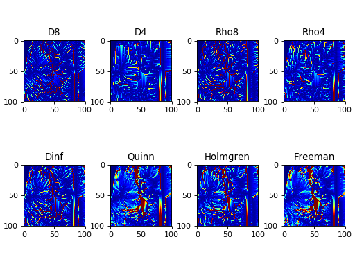
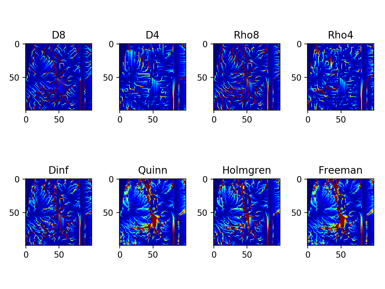
Side-by-Side Comparisons of Flow Metrics

(Source code, png, hires.png, pdf)

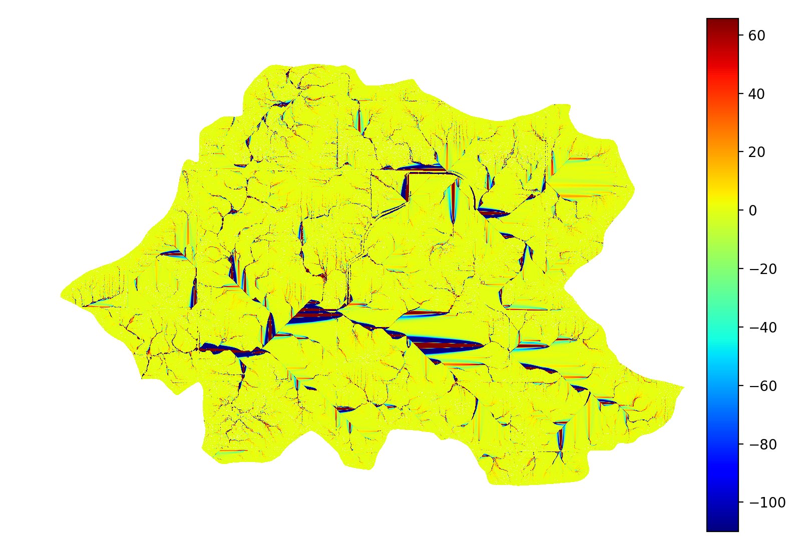
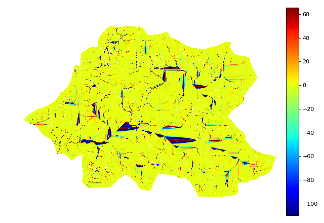
Note that Quinn (1991) and Freeman (1991) produce rather similar results; nonetheless, they are different:

(Source code, png, hires.png, pdf)

Accessing Flow Proportions Directly

In higher-level languages the foregoing flow proportions can be access via the flow proportions command, such as follows:

bprops = rd.FlowProportions(dem=beau, method='D8')

This command returns a matrix with the same width and height as the input, but an extra dimension which assigns each (x,y) cell 9 single-precision floating- point values.

The zeroth of these values is used for storing status information about the cell as a whole. If the 0th value of the area is 0 then the cell produces flow; if it is -1, then the cell produces no flow; if it is -2, then the cell is a NoData cell. The following eight values indicate the proportion of the cells flow directed to the neighbour corresponding to the index of that value where the neighbours are defined as in Flow Coordinate System.

For instance, the values:

0 0.25 0.25 0.25 0.25 0 0 0 0

direct 25% of a cell’s flow to the northwest, north, northeast, and east.

These values can be manipulated and used to generate custom flow accumulations.